In-class Exercise 4A: Preparing Spatial Interaction Modelling Variables

Overview

A well calibrated Spatial Interaction Model need conceptually logical and well prepared propulsiveness and attractiveness variables. In this in-class exercise, you will gain hands-on experience on preparing propulsiveness and attractiveness variables require for calibrating spatial interaction models. By the end of this in-class exercise, we will be able to:

• perform geocoding by using SLA OneMap API,

• convert an aspatial data into a simple feature tibble data.frame,

• perform point-in-polygon count analysis, and

• append the propulsiveness and attractiveness variables onto a flow data.

Getting Started

To get started, the following R packages will be loaded into R environment:

pacman::p_load(tidyverse, sf, httr,
               tmap)

Counting number of schools in each URA Planning Subzone

Downloading General information of schools data from data.gov.sg

We download General information of schools data set of School Directory and Information from data.gov.sg.

Geocoding using SLA API

Address geocoding, or simply geocoding, is the process of taking a aspatial description of a location, such as an address or postcode, and returning geographic coordinates, frequently latitude/longitude pair, to identify a location on the Earth’s surface.

Singapore Land Authority (SLA) supports an online geocoding service called OneMap API. The Search API looks up the address data or 6-digit postal code for an entered value. It then returns both latitude, longitude and x,y coordinates of the searched location.

The code chunks below will perform geocoding using SLA OneMap API. The input data will be in csv file format. It will be read into R Studio environment using read_csv function of readr package. A collection of http call functions of httr package of R will then be used to pass the individual records to the geocoding server at OneMap.

Two tibble data.frames will be created if the geocoding process completed successfully. They are called found and not_found. found contains all records that are geocoded correctly and not_found contains postal that failed to be geocoded.

Lastly, the found data table will join with the initial csv data table by using a unique identifier (i.e. POSTAL) common to both data tables. The output data table will then save as an csv file called found.

url<-"https://www.onemap.gov.sg/api/common/elastic/search"

csv<-read_csv("data/aspatial/Generalinformationofschools.csv")

Rows: 346 Columns: 31
── Column specification ────────────────────────────────────────────────────────
Delimiter: ","
chr (31): school_name, url_address, address, postal_code, telephone_no, tele...

ℹ Use `spec()` to retrieve the full column specification for this data.
ℹ Specify the column types or set `show_col_types = FALSE` to quiet this message.

postcodes<-csv$`postal_code`

found<-data.frame()
not_found<-data.frame()

for(postcode in postcodes){
  query<-list('searchVal'=postcode,'returnGeom'='Y','getAddrDetails'='Y','pageNum'='1')
  res<- GET(url,query=query)
  
  if((content(res)$found)!=0){
    found<-rbind(found,data.frame(content(res))[4:13])
  } else{
    not_found = data.frame(postcode)
  }
}

Next, the code chunk below will be used to combine both found and not_found data.frames into a single tibble data.frame called merged. At the same time, we will write merged and not_found tibble data.frames into two separate csv files called schools and not_found respectively.

merged = merge(csv, found, by.x = 'postal_code', by.y = 'results.POSTAL', all = TRUE)
write.csv(merged, file = "data/aspatial/schools.csv")
write.csv(not_found, file = "data/aspatial/not_found.csv")

Tidying schools data.frame

In this sub-section, we import schools.csv into R environment and at the same time tidying the data by selecting only the necessary fields as well as rename some fields.

schools <- read_csv("data/aspatial/schools.csv", show_col_types = FALSE) %>%
  rename(latitude = "results.LATITUDE",
         longitude = "results.LONGITUDE")%>%
  select(postal_code, school_name, latitude, longitude)

New names:
• `` -> `...1`

Converting an aspatial data into sf tibble data.frame

Next, we will convert schools tibble data.frame data into a simple feature tibble data.frame called schools_sf by using values in latitude and longitude fields.

This is done using the st_as_sf() of sf package.

schools_sf <- st_as_sf(schools, 
                       coords = c("longitude", "latitude"),
                       crs=4326) %>%
  st_transform(crs = 3414)

Plotting a point simple feature layer

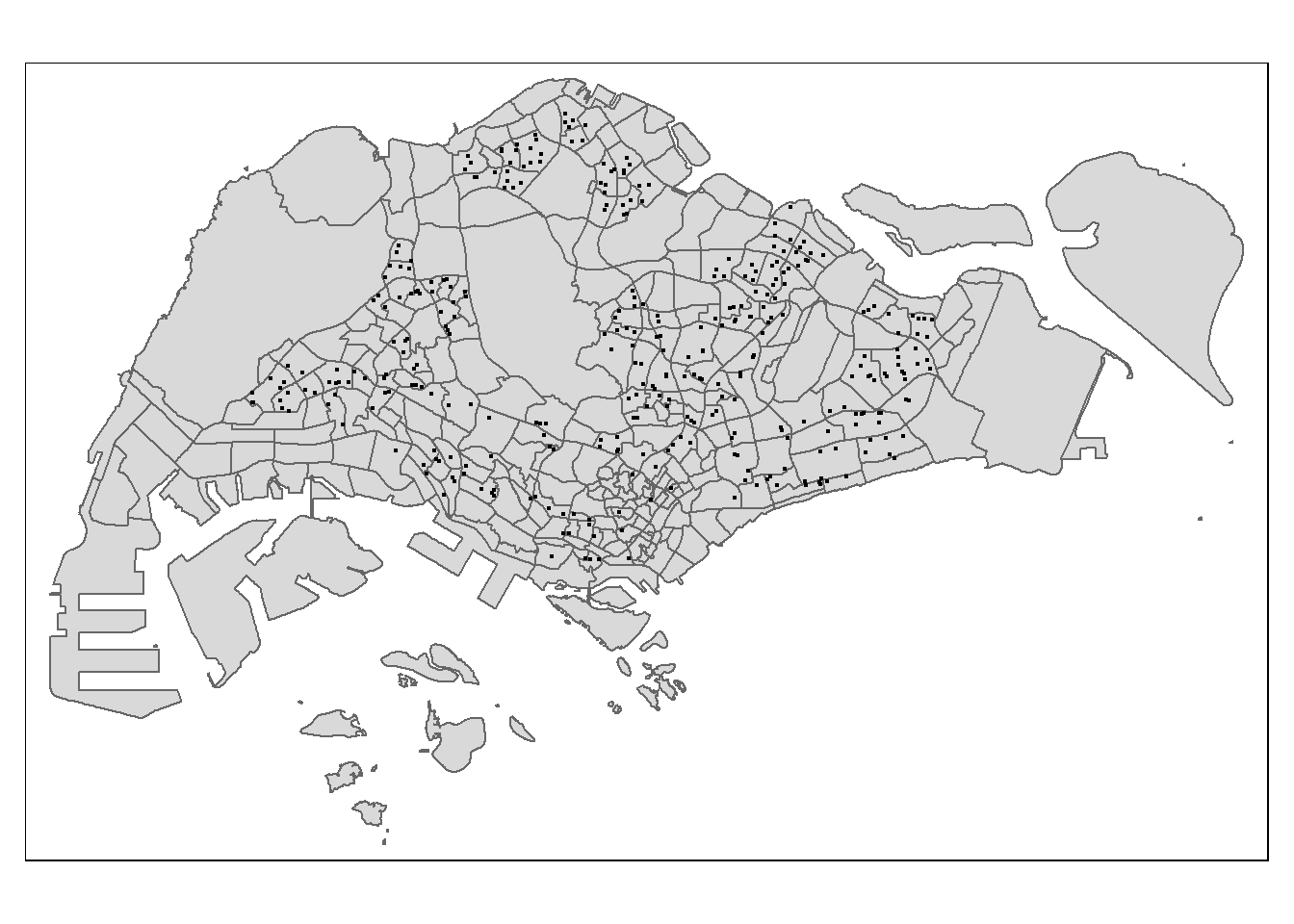
To ensure that schools sf tibble data.frame has been projected and converted correctly, you can plot the schools point data for visual inspection.

First, let us import MPSZ-2019 shapefile into R environment and save it as an sf tibble data.frame called mpsz.

mpsz <- st_read(dsn = "data/geospatial/",
                layer = "MPSZ-2019") %>%
  st_transform(crs = 3414)

Reading layer `MPSZ-2019' from data source 
  `C:\PeiShan0502\ISSS624\In-class_Ex4\data\geospatial' using driver `ESRI Shapefile'
Simple feature collection with 332 features and 6 fields
Geometry type: MULTIPOLYGON
Dimension:     XY
Bounding box:  xmin: 103.6057 ymin: 1.158699 xmax: 104.0885 ymax: 1.470775
Geodetic CRS:  WGS 84

We create a point symbol map showing the location of schools with OSM as the background map.

tmap_options(check.and.fix = TRUE)
tm_shape(mpsz) +
  tm_polygons() +
tm_shape(schools_sf) +
  tm_dots()

Warning: The shape mpsz is invalid. See sf::st_is_valid

Performing point-in-polygon count process

Next, we will count the number of schools located inside the planning subzones.

mpsz$`SCHOOL_COUNT`<- lengths(
  st_intersects(
    mpsz, schools_sf))

summary(mpsz$SCHOOL_COUNT)

   Min. 1st Qu.  Median    Mean 3rd Qu.    Max. 
  0.000   0.000   0.000   1.054   2.000  12.000 

The summary statistics above reveals that there are excessive 0 values in SCHOOL_COUNT field. If log() is going to use to transform this field, additional step is required to ensure that all 0 will be replaced with a value between 0 and 1 but not 0 neither 1.

Data Integration and Final Touch-up

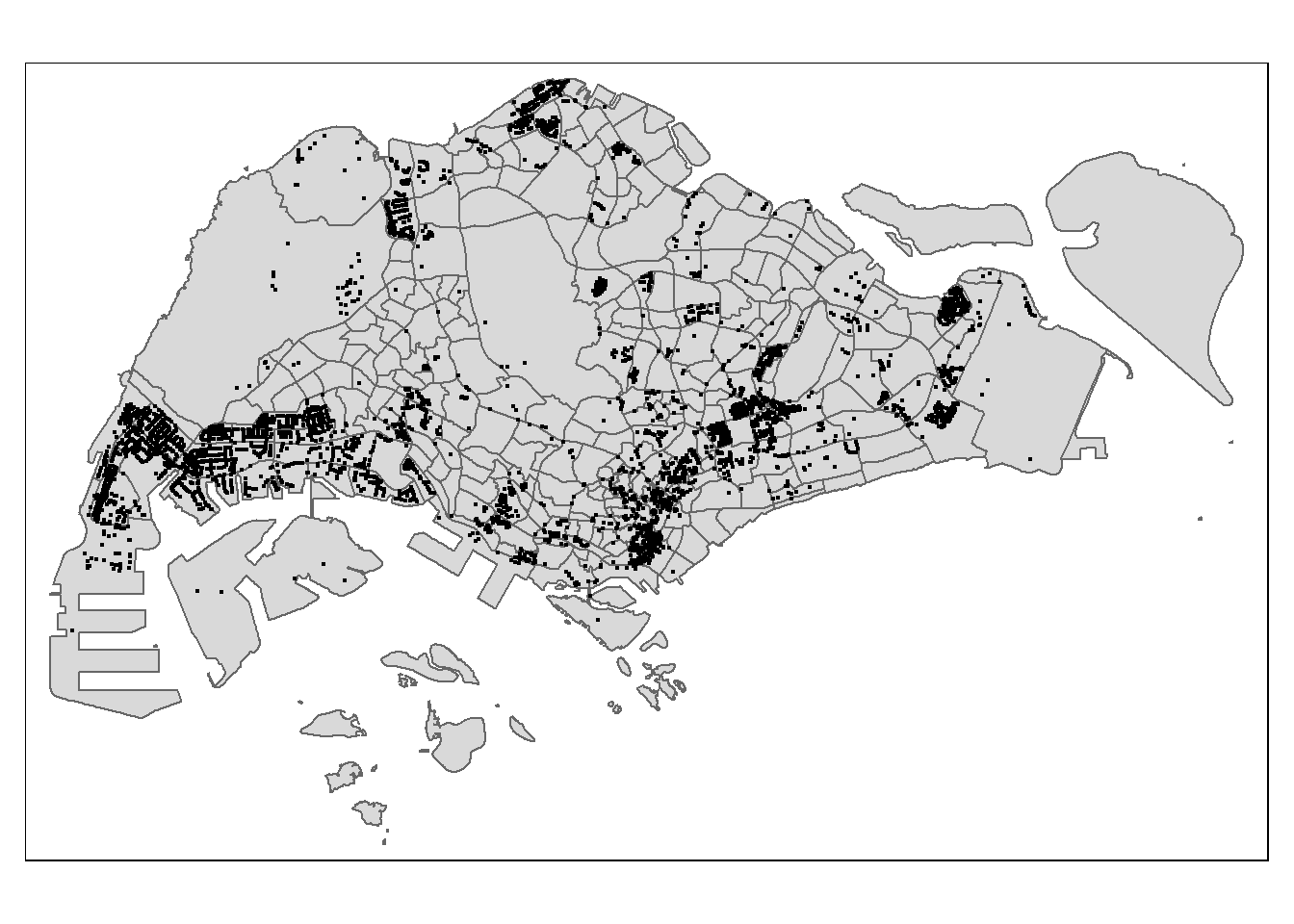
To count number of business points in each planning subzone:

business_sf <- st_read(dsn = "data/geospatial",
                      layer = "Business")

Reading layer `Business' from data source 
  `C:\PeiShan0502\ISSS624\In-class_Ex4\data\geospatial' using driver `ESRI Shapefile'
Simple feature collection with 6550 features and 3 fields
Geometry type: POINT
Dimension:     XY
Bounding box:  xmin: 3669.148 ymin: 25408.41 xmax: 47034.83 ymax: 50148.54
Projected CRS: SVY21 / Singapore TM

tmap_options(check.and.fix = TRUE)
tm_shape(mpsz) +
  tm_polygons() +
tm_shape(business_sf) +
  tm_dots()

Warning: The shape mpsz is invalid. See sf::st_is_valid

mpsz$`BUSINESS_COUNT`<- lengths(
  st_intersects(
    mpsz, business_sf))

summary(mpsz$BUSINESS_COUNT)

   Min. 1st Qu.  Median    Mean 3rd Qu.    Max. 
   0.00    0.00    2.00   19.73   13.00  307.00 

Now, we bring in the flow_data.rds saved after Hands-on Exercise 3:

flow_data <- read_rds("data/rds/flow_data.rds")
flow_data

Notice that this is an sf tibble data.frame and the features are polylines linking the centroid of origins and destination planning subzone.

append SCHOOL_COUNT and BUSINESS_COUNT into flow_data sf tibble data.frame:

mpsz_tidy <- mpsz %>%
  st_drop_geometry() %>%
  select(SUBZONE_C, SCHOOL_COUNT, BUSINESS_COUNT)

Now, we will append SCHOOL_COUNT and BUSINESS_COUNT fields from mpsz_tidy data.frame into flow_data sf tibble data.frame by using the code chunk below.

flow_data <- flow_data %>%
  left_join(mpsz_tidy,
            by = c("DESTIN_SZ" = "SUBZONE_C")) %>%
  rename(TRIPS = MORNING_PEAK,
         DIST = dist)

Checking for variables with zero values

Since Poisson Regression is based of log and log 0 is undefined, it is important for us to ensure that no 0 values in the explanatory variables.

In the code chunk below, summary() of Base R is used to compute the summary statistics of all variables in wd_od data frame.

summary(flow_data)

The print report above reveals that variables ORIGIN_AGE7_12, ORIGIN_AGE13_24, ORIGIN_AGE25_64, DESTIN_AGE7_12, DESTIN_AGE13_24, DESTIN_AGE25_64 consist of 0 values.

In view of this, code chunk below will be used to replace zero values to 0.99.

flow_data$SCHOOL_COUNT <- ifelse(
  flow_data$SCHOOL_COUNT == 0,
  0.99, flow_data$SCHOOL_COUNT)
flow_data$BUSINESS_COUNT <- ifelse(
  flow_data$BUSINESS_COUNT == 0,
  0.99, flow_data$BUSINESS_COUNT)

summary(flow_data)

Notice that all the 0 values have been replaced by 0.99.

Before we move on to calibrate the Spatial Interaction Models, let us save flow_data sf tibble data.frame into an rds file. Call the file flow_data_tidy.

write_rds(flow_data,
          "data/rds/flow_data_tidy.rds")